06. The Feedforward Process
Feedforward
In this section we will look closely at the math behind the feedforward process. With the use of basic Linear Algebra tools, these calculations are pretty simple!
If you are not feeling confident with linear combinations and matrix multiplications, you can use the following links as a refresher:
Assuming that we have a single hidden layer, we will need two steps in our calculations. The first will be calculating the value of the hidden states and the latter will be calculating the value of the outputs.
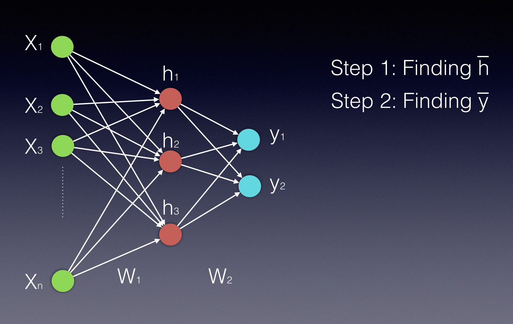
Notice that both the hidden layer and the output layer are displayed as vectors, as they are both represented by more than a single neuron.
Our first video will help you understand the first step- Calculating the value of the hidden states.
06 FeedForward A V7 Final
As you saw in the video above, vector h' of the hidden layer will be calculated by multiplying the input vector with the weight matrix W^{1} the following way:
\bar{h'} = (\bar{x} W^1 )
Using vector by matrix multiplication, we can look at this computation the following way:
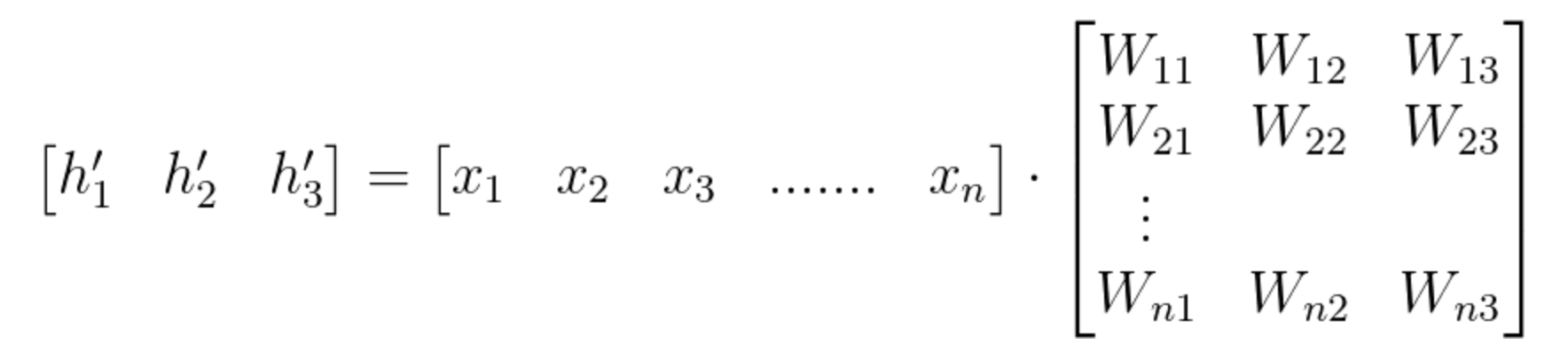
Equation 1
After finding h' , we need an activation function ( \Phi) to finalize the computation of the hidden layer's values. This activation function can be a Hyperbolic Tangent, a Sigmoid or a ReLU function. We can use the following two equations to express the final hidden vector \bar{h}:
\bar{h} = \Phi(\bar{x} W^1 )
or
\bar{h} = \Phi(h')
Since W_{ij}
represents the weight component in the weight matrix, connecting neuron i from the input to neuron j in the hidden layer, we can also write these calculations in the following way:
(notice that in this example we have n inputs and only 3 hidden neurons)
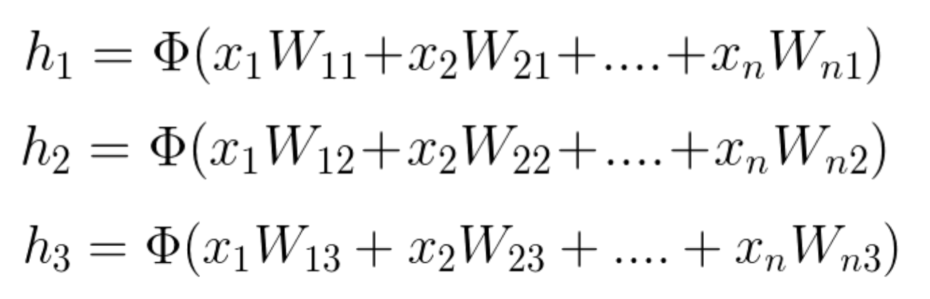
Equation 2
More information on the activation functions and how to use them can be found here
This next video will help you understand the second step- Calculating the values of the Outputs.
07 FeedForward B V3
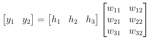
As you've seen in the video above, the process of calculating the output vector is mathematically similar to that of calculating the vector of the hidden layer. We use, again, a vector by matrix multiplication, which can be followed by an activation function. The vector is the newly calculated hidden layer and the matrix is the one connecting the hidden layer to the output.
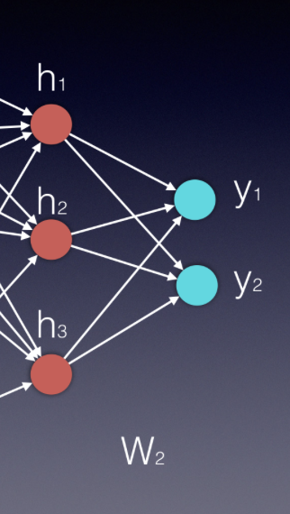
Essentially, each new layer in an neural network is calculated by a vector by matrix multiplication, where the vector represents the inputs to the new layer and the matrix is the one connecting these new inputs to the next layer.
In our example, the input vector is \bar{h} and the matrix is W^2, therefore \bar{y}=\bar{h}W^2. In some applications it can be beneficial to use a softmax function (if we want all output values to be between zero and 1, and their sum to be 1).
Equation 3
The two error functions that are most commonly used are the Mean Squared Error (MSE) (usually used in regression problems) and the cross entropy (usually used in classification problems).
In the above calculations we used a variation of the MSE.
The next few videos will focus on the backpropagation process, or what we also call stochastic gradient decent with the use of the chain rule.